RBF neural networks

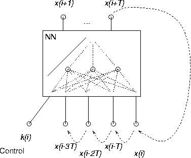
There are different topologies of neural networks that may be employed for time series modeling. In our investigation we used radial basis function networks which have shown considerably better scaling properties, when increasing the number of hidden units, than networks with sigmoid activation function [8]. As proposed by Verleysen et. al [11] we initialize the network using a vector quantization procedure and then apply backpropagation training to finally tune the network parameters. The tuning of the parameters yields an improvement factor of about ten in prediction error compared to the standard RBF network approach [8, 3]. Compared to earlier results [7] the normalization of the hidden layer activations yields a small improvement in the stability of the models.

The resulting network function for m-dimensional vector valued output is of the form

 

where represents the standard deviation of the Gaussian, the input and the centers are n-dimensional vectors and and are m-dimensional parameters of the network. Networks of the form eq. () with a finite number of hidden units are able to approximate arbitrary closely all continuous mappings [4]. This universal approximation property is the foundation of using neural networks for time series modeling, where we denote them as neural models. In the context of the previous section the neural models are approximating the systems prediction function.

To be able to represent instationary dynamics, we extend the network according to figure  to have an additional input, that enables the control of the actual mapping

 

  
Figure: Input/Output structure of the neural model.

This model is close to the Hidden Control Neural Network described in [2]. From the universal approximation properties of the RBF-networks stated above it follows, that eq. () with appropriate control sequence k(i) is able to approximate any sequence of functions. In the context of time series prediction the value i represents the actual sample time. The control sequence may be optimized during training, as described in [2], The optimization of k(i) requires prohibitively large computational power if the number of different control values, the domain of k is large. However, as long as the systems instationarity is described by a smooth function of time, we argue that it is possible to select k(i) to be a fixed linear function of i. With the preselected k(i) the training of the network adapts the parameters and such that the model evolution closely follows the systems instationarity.