Abstract

1. Introduction

The direct use by composers of temporal structure, however, poses a very different (although related) set of problems. A contemporary composer who wished to include gently accelerating accompaniment figures, as did Chopin, would be unlikely to consider the acceleration as a detail of execution, assuming that a performer should be able to guess the intention : this would be even more important if the accelerating figures contained varying numbers of notes.

The diversity of styles that coexist in contemporary music has, for better or worse, forced composers to communicate explicitly their intentions rather than imagining all performers to be familiar with their style and its associated performance practices. Therefore an intelligent compositional quantizer would search for a notation that clearly expresses the composers intention of a gentle acceleration. A traditional quantizer could, of course, produce this if it were allowed a large resolution (e.g. to the nearest 32nd note). This would however produce a complexity of notation that would be equally masking of the desired effect as would have been Chopin's solution (in either case you must be told that a gentle acceleration is desired since the written rhythms have not made that clear).

The compositional quantizer must search for a way to express the desired structure that is both accurate and simple enough to be understood. In order to succeed it must make use of the notational tools available to contemporary composer (e.g. changes of tempo and meters). This paper presents a prototype of a compositional quantizer : Kant.

The quantizer that we propose divides the task into several levels. We have strategies for proposing solutions at each of these levels, but require the guidance of a composer to choose from, add to and/or select various propositions. It is our feeling that musical notation must ultimately remain personal to every composer and thus each composer should be able to use our system to arrive at his own solution. We have tried to realize a system flexible at every level, so that even if a particular sequence is a poor fit with the tools at one level, the next level can compensate for any problems in the previous steps solution. The first step in quantifying a sequence is to divide that sequence into various sections which we call archi-measures. Each archi-measure will be notated in a single tempo or as a continuous accelerando or ritardando. The second step is to divide each archi-measure into segments which will correspond, more or less closely, to measures. This step will provide the metric structure as well as the tempo. Finally we must resort to a grid (similar to that of traditional quantizer possessing, however, a very different means of choosing the best result). All of these steps are performed from a single interface which allows interaction and guidance from the composer, permitting him to fine tune the first and second steps as well as the parameters for the last until an acceptable quantification has been found.

2. Solving local rhythmic complexity.

PatchWork ([AR 93], [LRD 93]) supplies a standard module performing basic quantification, which we have used to perform the final step of quantification within the beat. This module has been integrated and modified to serve as a transparent part of Kant's interface. Input to this module is a list of tempi, a list of measure signatures, a set of quantification constraints and a list of real durations to be quantified. Tempi and measure information are used to build a sequence of beats of (possibly) varying duration. Durations are then transformed into onset times which are distributed along the time axis and fall inside their corresponding beats, thus defining potential beat subdivisions. Each beat is then subdivided (i.e. triplet, quintuplet, etc.) independently, complying with the supplied constraints and according to both built-in and user definable criteria. Borderlines between consecutive quantized beats are further examined to identify the need of slurs. Quantized onset times are finally used to construct a tree structure of duration proportions. Lower level nodes in this tree represent rhythmic notation of beat subdivisions while higher level nodes refer to rhythmic notation of measures or set of measures. This hierarchical structure is the standard representation of a rhythm in PatchWork's music notation editors which we use to display the music.

The fundamental issue in this scheme is of course the particular criteria used to independently quantize each beat. The process begins by computing a set of potential integer divisors of the beat duration, which is simply the set of integers growing from the number of onsets falling inside the beat up to 32. Each of these defines a different pulse length. Each pulse length determines a grid for measuring the beat length. For each particular grid, onsets are moved to their nearest point on the grid and an error measure relating true and moved values of onsets is computed. Output is the set of moved onsets for the grid giving the least error.

The module has been programmed in such a way to easily accommodate different error measures. For each grid, a structure is constructed containing all the moved onsets, the number of onsets eliminated (i.e. falling on the same point in the grid) and a list of different error values. Each error value in the list is computed by a user-supplied or built-in function invocation. In the current implementation, three error values are used. The first one is the sum of the cubic ratios between duration intervals extracted from the true onsets and corresponding intervals extracted from the moved onsets. The second one is the simple Euclidean distance between the true onsets and the moved onsets. The third one is a subjective measure of the relative simplicity of different beat divisions. It is computed from the position of the grid in a user supplied table (in the current implementation we have defined the relative "complexity" of different subdivisions of the beat in the following order : 1, 2, 4, 3, 6, 8, 5, 7 etc. where a single division of the beat is the simplest possible notation and each successive number of divisions is increasingly complex).

These three measures are combined by the following procedure : two complete sets of structures are first computed. The first set is ordered according to the simplicity criteria. The second one is ordered according to the duration proportion criteria. In both sets, structures eliminating the least number of onsets are favoured. These structures are then further filtered according to a set of given constraints. The user can either impose or forbid particular subdivisions at any level of the rhythmic structure (sequence, measure, beat). Structures not complying with these constraints are eliminated from the sets.

The final choice of subdivision for each beat is made by taking the highest ranked choice in both sets and comparing their respective values for the Euclidean distance criteria, modified by scaling factors. The scaling factor for the first set is a user defined parameter w we call "precision", ranging from 0 to 1. Its complement (1-w) is used to scale the second set. The beat division whose scaled Euclidean distance is smallest is chosen.

When two events fall on the same point in the grid one of the events is eliminated by the quantification process, the corresponding duration is kept in a separate structure which also contains information on the position of the duration in the original event sequence. This information is later used by Patchwork's music notation editor to transform eliminated durations into grace notes attached to the note whose duration follows in the original sequence. Keeping track of eliminated onsets is particularly delicate in this quantification scheme due to the independent treatment of each beat.

This system, which on the surface seems quite complicated grew out of purely musical reasoning. Our first concern was to find an error measure which was extremely accurate in a musical sense. Standard Euclidean measures were flawed by their simple cumulative procedure: in a musical structure error needs to be as evenly distributed as possible. An Euclidean algorithm will give the same result to a quantification containing a large distortion followed by two very small ones as it would to three medium distortions; the second, however would be musically preferable. The choice we made was to us a function based on the duration ratios (already more perceptually relevant than simple onset times -- see [DH 92] for a discussion on onset-quantification versus duration-quantification) which made use of a cubic function. The form of this function which provides a relatively flat plateau followed by a steep rise is tolerant of errors within the flat central area while heavily penalizing larger distortions. In parallel to this measure of 'accuracy' we needed another procedure, capable of deciding the complexity of each solution. This would permit us to find a solution that might be only slightly less accurate while being much simpler. The problem of choosing between the two lists of solutions necessitated a third (and in a sense objective) algorithm: for this we went back to Euclidean distance. The ordering which has been determined by the other algorithms prevent the occurrence of the worst case Euclidean error described above and, thus, in the role of arbiter it is quite effective. The Euclidean distance of the solutions proposed by the two preceding criteria is scaled to favour precision or complexity. The result whose scaled Euclidean measure is smaller is chosen. This system has great advantages over traditional complexity controlling schemes which make use of a maximum number of subdivisions parameter in that it is capable of choosing a complex solution (such as a septuplet) when the data requires, while still being able to simplify a non-essentially complex result such a quarter note of a septuplet followed by a dotted eighth of a septuplet into two eighth notes.

3. Solving global rhythmic complexity.

3.1. Polyphony.

3.2. Segmentation.

Usual concepts have proven to be inefficient in the case of complex duration patterns : the biggest problem arises from the fact that salient perceptual sub-structures, like disjoint clusters of events, or synchronous onset times occurring inside an otherwise tangled polyphony, are not adjusted to visually (and musically) salient places (i.e. beat or measure onset) in the resulting score. Tempo and meter recognition can be based on procedures (e.g. autocorrelation) that estimate the combined periodicities of events. This works fine in the case where a pre-existing score (or its interpretation), possessing a well defined, periodic, beat/meter grid, is analyzed [Brown 93]. However, in thecase of contemporary composition, it can not give a guarantee that higher level event subsets, scattered in a non-periodic way over the score, and nevertheless crucial to the understanding of the musical structure, will be correctly aligned with the beat/meter grid.

In order to bypass this obstacle, we hierarchize the events by giving a non null weight to those of them that surround salient substructures, considering them as articulation events whose onsets or outsets will determine a borderline separating adjacent sets of events. This segmentation of the input sequence will have two distinct functions :

• 1. cut out the sequence into archi-measures (contiguous subsequences, each submitted to a single tempo)
• 2. cut out the archi-measure into segments.

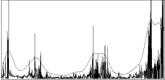
For each of these levels of segmentation, different strategies will be proposed to the user. Some of these will be easily understandable if we represent the event stream as a graph where the x-axis represents an index i through the event stream and the y-axis represents the duration di for each of these events. An example of such a graph is presented in Figure 1. It shows a six mn long piano improvisation captured on a Yamaha Midi Piano, with about 1000 events.

Figure 1.

By simply smoothing that curve we obtain a fair idea of the distribution of event density in time. Regions centered at the minima and maxima are interesting for higher level segmentation (archi-measures). Region borderlines can be obtained by computing the second order derivative. At this step, small hand adjustments still have to be made on the precise borderline positions.

Once archi-measures have been determined, they must, in turn, be segmented into measures.

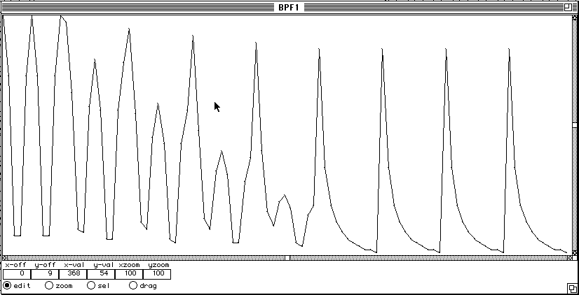
Figure 2.

Figure 2 and 3 show an archi-measure extracted from an other sequence computed by composer Tristan Murail. Figure 2 shows the duration plot and figure 3 shows the rhythm in proportional notation. This series of durations was obtained by sampling a sine wave (this produces durations which accelerate and then decelerate periodically) then deforming step by step this form until it becomes an exponential curve (a fairly close model for an accelerando as interpreted by a musician). The exponential form is repeated 4 times at the end of sequence.

A significant peak structure is visible. The maxima correspond to long durations that separate patterns of shorter duration. These maxima give birth to agogic accents that are clearly perceived as articulations. The minima help to localize sudden increase of the event density that tend to be perceived as groups. The problem is that segment border should be aligned on the left side of the groups. This is achieved by computing a density function that associates with each event the number of events that follow within a given time window. In order to favour the recognition of regions of high density, it is even better to sum the inverses of the durations of the events falling inside the window. Then the maxima of the density function (eventually smoothed) are extracted to determine the segment positions. Figure 3 shows the two segmentations, using the symbol '*' for the maxima and 'o' for the minima.

Figure 3.

(defun agcd (values tolerance)
  "approximate gcd with backtracking"
  (labels 
    ((grid-above (val) (* val (1+ tolerance)))
     (grid-below (val) (- val (* val tolerance)))
     (gcd-try (values gcd-min gcd-max)
       (when (<= gcd-min gcd-max)
         (if (null values)
           (/ (+ gcd-min gcd-max) 2.0)
           (let* ((val-below (grid-below (first values)))
                  (val-above (grid-above (first values)))
                  (quo-min (ceiling (/ val-below gcd-max)))
                  (quo-max (floor (/ val-above gcd-min))))
             (loop for quotient from quo-min upto quo-max
                   for gcd-interval =
                   (gcd-try (rest values)
                            (max gcd-min (/ val-below quotient))
                            (min gcd-max (/ val-above quotient)))
                   when gcd-interval do (return-from gcd-try gcd-interval)))))))
    (gcd-try values .1 (grid-above (first values)))))

3.3. Tempo extraction.

A unit duration (i.e. a beat duration) will be computed as an approximate greatest common divisor (agcd) of the list of segment durations li = d(Si). We have obtained the best results with an algorithm that was previously conceived in order to compute the virtual fundamental of a discrete spectrum given as a list of frequencies (see [ACM 85] and algorithm in figure 4). It is used there unchanged, the frequencies being replaced by the segment durations, and the virtual fundamental being interpreted as the beat duration.

A first, temporary, beat P1 is computed. P1 = agcd (li , tolerance1). round (li  / P1) is then the number of iterations of P1 inside segment Si (note that (li  / P1) is a real number whose fractional part denotes a residue in the segment). A second, eventually longer beat P2 is then computed. P2 = agcd (li  / P1, tolerance2). The final value retained for the pulsation is P = P1 * round (P2).

agcd yields an interval of values which length depends on the tolerance factor and of the magnitude of values li . Tolerance1 is usually small (i.e. 3% to 15%) thus leading to a narrow interval for P1, while tolerance2 can be bigger (i.e. 10 % to 20%) as P2 is computed on smaller numbers. Furthermore P2 is rounded, thus it converges towards a small set of integer values. This two-level tolerance system is an optimisation that leads quickly to a reasonable value of P. The process could be otherwise achieved in a single pass by enlarging the tolerance, but would then yield a bigger interval of real values that would be tedious to explore. The tempo extraction module tries several values for tolerance1 and tolerance2 inside a pre-defined range and using a pre-defined step. This generates a list of values for P which are converted into conventional tempo indications, expressed as an integer number of quarter notes per minute. In general, results converge around a limited number of possible tempi.

3.4. Segment scaling.

This difference is eliminated by applying a coefficient round(ki) * P / li  to every duration inside segment Si, moving the onset times accordingly. Duration proportions are thus conserved inside the segments, that are independently stretched or shrunk depending on ki.

This step reduces the effects of the two greatest problems posed by traditional quantification strategies.

The first is shifting of the durations relative to the beat grid. The coordination between events and beat is realigned at the beginning of each measure. Thus we avoid the accumulation of a greater and greater amount of error as the sequence progresses.

The second problem is that of structurally perceptible local distortions (e.g. a shorter note followed by a longer note within an accelerando). The fact that segmentation isolates structurally important groups of events such as an acceleration, allows us to treat them as an undistorded whole rather than distributing the error where it happens to fall. This approach is consistent with psycho-acoustic findings that an acceleration or other recognizable structure lasting for example 3 seconds is perceptually indistinguishable from the same structure lasting 3.2 seconds. However, a perturbation of a single note within that structure by only a few hundredth of a second may be perceived.

In terms of the total duration of the sequence, experience has shown that the segment transformations described above tend to occur statistically equally in both directions resulting in an overall sequence duration close to the original.

Figure 5 details the 4 steps.

3.5. local quantification.

The relative length of measures has no other meaning than to express the boundaries of musical structures and thus it may be necessary for the composer to divide long measures into several parts or to regroup small measures. In any case these operations will leave intact the beat/event structure.

Figure 6 shows the final output for the example discussed above, as computed by Kant. In Figure 7, a few segment borders have been slightly moved by hand, using the Kant editor, in order to improve the result.

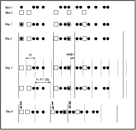
Figure 5.

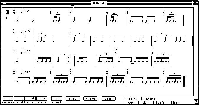
Figure 6.

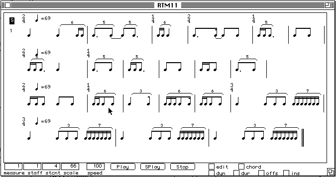
Figure 7.

4. Summary.

Kant exists now as a new editor box in PatchWork. Available functionalities are :display of the sequence in proportional duration and in duration plot, archi-measure segmentation using density function or interactive manual input (this can be achieved in both representations of the sequence. The two views are mutually informed of changes), measure segmentation using one of five criteria (maxima, minima, chords -- this method, not described in the paper, tracks almost synchronous events in the case of a polyphonic sequence -- rests, manual segmentation), interactive editing of the articulation points between segments (move or delete), boolean combination of segmentation criteria.

The agcd algorithm has been recently improved in order to accept a gcd that divides almost every component, the remaining ones being divided by the half or the third of the gcd. The practical meaning is that Kant can generate measures like 5/8 and 7/8 or, as an option can produce the sort of fractional measures used by some contemporary composers (e.g. 3/4 + 1/3).

Further possible improvements include increasing the collection of segmentation criteria (notably by the detection of durational patterns of musical significance or non local repetition of patterns).

5. Acknowledgements.

6. References.

[Brown 93] Brown J.C. Determination of the meter of musical score by autocorrelation. J.Acoust.Soc.Am. 94. 1953-1957. 1993.

[DH 91] P. Desain, H. Honing (1991). The Quantization Problem : Traditional and Connectionist Approaches. in M. Balaban, K. Ebcioglu & O. Laske (Eds) Understanding Music with AI : Perspectives on Music Cognition, pp 448-463, The AAAI Press, 1992.

[LRD 93] M. Laurson, C. Rueda, J. Duthen. The Patchwork Reference Manual, IRCAM, 1993. [an error occurred while processing this directive]