Xavier Rodet, IRCAM
Additive is an Analysis-Synthesis package aimed at representing sound signals, modifying and resynthesizing them. It runs at IRCAM on Unix DEC and SGI worksations. The list of contributors includes P. Depalle, G. Garcia, X. Rodet, R. Woehrmann and I. Perry. A version of additive is also implemented on Macintosh, but the present documentation is written for the Unix version.
The underlying model is in terms of sum of sinusoids
(called partials) with time-varying frequencies, amplitudes and
phases. These time-varying values are called parameters. Therefore,
the result out of an Additive analysis is a parameter file containing these
time-varying values. In fact, there are several different analysis steps. The
first one is called Pitch or Fundamental Frequency (f0, i.e.
f-zero) analysis and produces an f0 parameter file with the file
name extension .f0.sdif (see SDIF) or .f0.
The second one makes an estimation of partial trajectories,
i.e. of the time evolution of frequencies, amplitudes and phases of partials.
It produces a partial parameter file designated with the file name extension .part.sdif or
.format or .fmt (e.g.: file.part.sdif or file.format or file.fmt).
Another analysis step estimates the spectral envelope of sinusoidal partials thanks to the the
discrete cepstrum method by using the program estimate.
The resulting file is an .penv.sdif or .penv file (see below). For
information about spectral envelope estimation, see estimate.
The synthesis stage takes a partial parameter file as input and computes
a synthetic signal (signal.synth.sf or signal.synth.aiff) which is
close to the original signal which has been
analysed to produce the partial parameter file as long as the parameter
file is not modified.
Another stage is the computation of a residual
signal (signal.noise.sf or signal.noise.aiff), named
noise for simplicity, as the difference between
the original signal and the synthetic signal.
The spectral envelope of the noise (.nenv.sdif or .nenv file) can
also be calculated (it also relies on estimate).
Modifications of frequencies, amplitudes and time informations are not difficult and allow a large variety of sound transformations.
The simplest analysis and synthesis of a sound-file, say test.aiff, is as follows:
additive -0 -A -Z -D -S test.aiff
It creates a subdirectory ADDtest in the directory $DATADIR (see below) and the files history, test.f0.sdif and test.part.sdif in the directory ADDtest. It creates sound files test.synt.aiff and test.noise.aiff in the directory $SFDIR (see below).
Additive uses the Unix environment variable $SFDIR to designate the file directory where sound files are to be found or written to. If a sound file name is given with a relative path, this path is supposed to be relative to the directory registered in $SFDIR. If a sound file name is given with an absolute path, the SFDIR directory is ignored. The variable $SFDIR can be set by using the Cshell command setenv. Example:
setenv SFDIR /user/my_group/my_name/sound_dir/
Additive recognizes and can write two types of sound-file formats, the AIFF/AIFF-C, with extension .aiff and the Ircam format with extension .sf. The AIFF format is the one used by Apple and SGI. Additive handles 8/16/24/32-bit two's complement integer samples (without compression). The Ircam format comprises 16 bit two's complement integer (short) samples and 32 bit floating point samples. A set of programs is available at IRCAM for sound management and playing: fromsf, tosf, querysf, playsf, normsf, peaksf, diffsf, sfmix and xspect. To get some information about these programs, use the option -h (e.g. fromsf -h) or the man command (e.g. man fromsf).
Additive uses the Unix environment variable
$DATADIR to designate the file directory where parameter files directories
are to be found or written to. By default, DATADIR is set to SFDIR. The
parameter file directory name is composed of the prefix ADD followed by
the name of the sound without its .sf or .aiff extension. A file named
history is also written in the ADD<name> directory. It
contains the trace of the successives analysis performed on the sound file
<name>.sf or <name>.aiff.
For example, the analysis of the sound flute.sf
may produce the parameter files history, flute.f0.sdif and flute.part.sdif
in the directory ADDflute in the $DATADIR directory.
There are several types of parameter files. The first one with extension .f0.sdif or .f0 (according to the -f0ascii option, see below) contains the fundamental frequency of the analysed sound.
Here is the "text" conversion of an .f0.sdif file :
SDIF

1NVT
{
StreamID        0;
Date    Wed_Jun__7_15.58.58_2000_;
TableName       GenericBreakPointFunction;
WrittenBy       Pm_Version_1.2.2;
}


SDFC

1FQ0    1       0       0.02
  1FQ0  0x0004  1       1
        117.934

1FQ0    1       0       0.03
  1FQ0  0x0004  1       1
        74.1056

1FQ0    1       0       0.04
  1FQ0  0x0004  1       1
        98.8639
        .
        .
        .
ENDC
ENDF
The .f0 file is an ASCII file with two columns containing the time in seconds of the analysed frames and the corresponding fundamental frequencies in Hertz:
time_in_secs_1     f0_value_1
time_in_secs_2     f0_value_2
time_in_secs_3     f0_value_3
    .                  .
    .                  .
    .                  .
Here is an example of an .f0 file :
0.020000        117.934227
0.030000        74.105606
0.040000        98.863930
   .               .
   .               .
   .               .
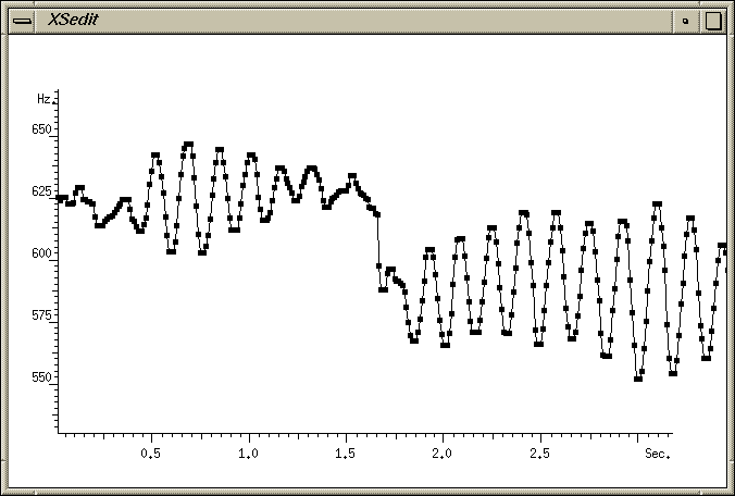
Such a file can be graphically displayed with programs such as gnuplot, xgraph (runs on SGIs only) and XSedit. Here is a graphic display of a .f0 file using XSedit (XSedit < name.f0):
The second type of parameter file with extension .part.sdif or .format or .fmt (according
to the -ascii option and the -bin option, see below) contains the parameters of the
sound partials. The .part.sdif file is an
Here is the "text" conversion of an .part.sdif file :
SDIF

1NVT
{
StreamID        0;
Date    Wed_Jun__7_15.12.41_2000_;
TableName       SinusoidalTracks;
WrittenBy       Pm_Version_1.2.2;
}


SDFC

1TRC    1       0       0
  1TRC  0x0004  306     4
        1       111.107 0       2.35351
        2       240.395 0       -2.37539
        3       344.269 0       3.11186
        .       .       .       .
        .       .       .       .
        .       .       .       .

1TRC    1       0       0.02
  1TRC  0x0004  306     4
        1       111.107 6.08317e-05     -2.53392
        2       240.395 1.06125e-05     2.70081
        3       344.269 9.63689e-06     2.3917
        .       .       .       .
        .       .       .       .
        .       .       .       .

1TRC    1       0       0.03
  1TRC  0x0004  306     4
        1       95.4705 8.15562e-05     -1.939
        2       162.541 1.45304e-05     -1.88946
        3       219.027 1.82551e-05     -1.48168
        .       .       .       .
        .       .       .       .
        .       .       .       .

ENDC
ENDF
The .format file is an ASCII file containing the successive frame data. Each frame data begins with one line containing the number N of detected partials during this frame and the frame time in seconds. This line is followed by the N partial data, i.e. index, frequency, amplitude and phase. frequency is in Hertz, amplitude is the amplitude of the sinusoid, and phase is between -Pi and +Pi. The index is the harmonic number of the partial for the given fundamental frequeny:
number_of_partials_frame_1 frame_1_time_in_secs
index_1    frequency_1      amplitude_1        phase_1
index_2    frequency_2      amplitude_2        phase_2
index_3    frequency_3      amplitude_3        phase_3
   .            .               .                 .
   .            .               .                 .
   .            .               .                 .
index_N    frequency_N     amplitude_N        phase_N
number_of_partials_frame_2 frame_2_time_in_secs
index_1    frequency_1      amplitude_1        phase_1
index_2    frequency_2      amplitude_2        phase_2
index_3    frequency_3      amplitude_3        phase_3
   .            .               .                 .
   .            .               .                 .
   .            .               .                 .
Here is an example of a .format file :
306     0.000000
1       111.107079      0.0000000000    2.353510
2       240.395111      0.0000000000    -2.375390
3       344.269196      0.0000000000    3.111856
.       .               .               .
.       .               .               .
.       .               .               .

306     0.020000
1       111.107079      0.0000608317    -2.533919
2       240.395111      0.0000106125    2.700808
3       344.269196      0.0000096369    2.391699
.       .               .               .
.       .               .               .
.       .               .               .

306     0.030000
1       95.470520       0.0000815562    -1.938999
2       162.541412      0.0000145304    -1.889464
3       219.026627      0.0000182551    -1.481677
The .fmt file is the binary version (-bin option) of the .format file but is organised in a different way. It is a succession of 32 bits floating point numbers, so that you can look at it with the Unix od command. Each frame data begins with the frame time in seconds and the number N of detected partials during this frame, note that both are floating point numbers! They are followed by the N partial indexes (floating point numbers!), then the N frequencies , the N amplitudes and the N phases. The index is the harmonic number of the partial for the given fundamental frequeny:
frame_1_time_in_secs number_of_partials_frame_1 index_1 index_2 index_3 ...
... index_N frequency_1 frequency_2 frequency_3 ...
... frequency_N amplitude_1 amplitude_2 amplitude_3 ... amplitude_N
phase_1 phase_2 phase_3 ... phase_N frame_2_time_in_secs
number_of_partials_frame_2 index_1 index_2 index_3 ...
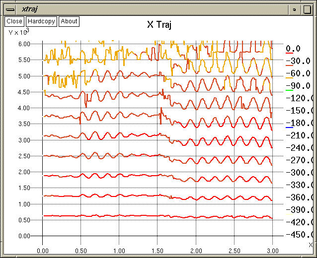
Files of partials can be graphically displayed by using the program xtraj which runs on SGI only:
The third type of parameter files with extension .penv.sdif or .penv (according
to the -Ea option, see below) contains spectral envelope
parameters of sinusoidal partials. The .penv.sdif file is an
Here is the "text" conversion of the .penv.sdif file :
The .penv file is an ASCII file containing the successive frame
data. The file begins with a line containing the number NumEnv of
envelope points of each frame, the maximum frequency MaxFreq of estimation
(see option -EM) and frequency step (MaxFreq/NumEnv). Then, the file contains amplitude data
of each frame :
The fourth type of parameter files with extension .nenv.sdif or .nenv (according
to the -Ea option, see below) contains spectral envelope
parameters of the noise. The .nenv.sdif file is an
Here is the "text" conversion of the .nenv.sdif file :
There also exists another type of file, the .pics.sdif file, but this
is rarely used (see below option -P). The program is started by typing: where options is a list of blank separated options. In particular
the option -h gives the following brief help: This option, -0 without argument, forces the computation of the
fundamental frequency f0 even if there is a <sound-name>.f0.sdif file
in the ADD<sound-name> directory. The result is a fundamental frequency
<sound-name>.f0.sdif file in the ADD<sound-name> directory. In the
absence of this option, f0 would not be recomputed if there exist already
a <sound-name>.f0.sdif file in the ADD<sound-name> directory. This
feature allows one to use an existing .f0.sdif file or to modify it before doing
the partial analysis. Modification of a .f0 file can be done with any text
editor (such as emacs or vi) or with a graphic program such
as XSedit, and conversion from/to .f0.sdif can be done with pmconvert. This option, -A without argument, causes the computation of partial
trajectories. This is done in the three following steps: The result is a partial parameter file <sound-name>.part.sdif or .format
file (according to the option -ascii, see below) in the ADD<sound-name>
directory. This option, -P without argument, is rarely used, only if for
some application you want the spectral peaks. This option causes the computation
of spectral peaks on each successive frame of signal. The result is a peak
parameter file <sound-name>.pics.sdif in the ADD<sound-name> directory.
The .pics.sdif file is an SDIF file.
Here is the "text" conversion of the .pics.sdif file :
This option, -Z without argument, causes the computation of a
synthetic signal as the sum of partial with the parameters found in the
<sound-name>.sdif or .format or .fmt in the ADD<sound-name> directory.
The result is a sound file <sound-name>.synt.sf or .aiff, the extension
and the sample rate being the same as for the sound-file name given after
the option -S (see below). This option, -D without argument, causes the computation of a
residual signal, named noise for simplicity, as the difference between
the original signal and the synthetic signal. If all sinusoidal partials
have been found in the partial analysis stage, only non-sinusoidal, i.e.
noise-like sound should remain in this residual signal. The result is a
sound file <sound-name>.noise.sf or .aiff, the extension and the
sample rate being the same as for the sound-file name given after the option
-S (see below). By default, the format of the fundamental frequency file is as
described above (.f0 and .f0.sdif files). The
option -L causes the fundamental frequency file format to be extended
with more information (see the command f0 -h and f0). By default, for security, the user is prompted when an existing file
risks to be overwritten. Option -V causes this security to be omitted. By default, the partial parameter file is written
in SDIF (.part.sdif) in the format indicated above. The -bin
option causes the partial parameter file to be written
in binary (.fmt extension).
By default, the partial parameter file is written
in SDIF (.part.sdif) in the format indicated above. The -ascii
option causes the partial parameter file to be written
in ASCII (.format extension).
By default, the fundamental frequency file is written
in SDIF (.f0.sdif) in the format indicated above. The -f0ascii
option causes the fundamental frequency file to be written
in ASCII (.f0 extension). By default, the estimated f0 trajectory is smoothed to avoid spurious
deviations. This flag omitts smoothing. This option simply states that the output file be played after synthesis.
This option specifies that the syntheis stage be performed ignoring
values calculated for phase of each partial.
Specifying this flag means that the fft file produced by SVP be saved as
an output file rather than being discared as is normal.
The following options want an argument after the letter. Note that there
shall be a space at least between the letter and its following argument. This indicates the name (eventually with a path) of the Sound file to
be analysed. Example -S test.aiff. Relative paths will be searched in SFDIR, except for paths starting
with '~', './', or '../', and of course absolute paths. Sound files should
be AIFF or sf sound files (see Sound Files and Parameter Files
above). The name of the sound itself, i.e. what precedes
the postfix .aiff or .sf, is used to build a directory by using the prefix
ADD, e.g. ADDname which is created in the DATADIR directory (see Sound
Files and Parameter Files above). It can NEVER be omitted. In particular, when performing synthesis
from an existing parameter file, say <name>.fmt, the program
additive wants to find a file <name>.sf in
the $SFDIR directory, a directory ADD<name> in the
$DATADIR directory and a file <name>.fmt in the ADD<name> directory.
This can be tedious to install. For synthesis, one can directly use the
syntadd program to perform the synthesis. Note that syntadd
writes floating-point samples on its standard output and should be piped
into tosf in order to produce a sound-file. See syntadd -h
and tosf -h for more details. Example: This is the time in seconds at which to start the analysis in the sound
file. Example -b 1.32. The default is 0. This is the time in seconds at which the analysis shall end in the sound
file. Example -e 1.32. The default is the end of the file.
Usually you dont have to set this number, the program calculates it
for you as the power of two greater or equal to the number of samples in
the analysed frame of signal. Use it only if you understand what it does.
It is the size of the FFT applied on the signal frame after zero padding.
It should be a power of two and greater or equal to the number of samples
in the analysed frame of signal. The size in seconds of the signal window (or frame) which is analysed
by FFT at each step. Example -M 0.022. The default is 0.04
seconds. In order that spectral peaks appear separated in the FFT analysis,
the signal window size should be at least equal to 3 time the inverse of
the smaller distance in Hertz between the peaks or partials which should
be detected in the analysis. For instance if f0_min is the minimum fundamental
frequency in the file, the harmonic partials are separated by f0_min at
least. Therefore, the signal window size should be at least equal to 3/f0_min.
For security, it is better to take 3.5/f0_min. Larger windows provide better
peak separation and safer partial parameter estimation but tend to smooth
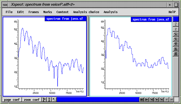
rapid parameter evolution. The following image shows spectra computed on
windows of size 4/f0 (left) and 3/f0 (right). After each frame analysis, the signal window (or frame) is advanced
by this step. Example -I 0.005. Lower limit and upper limit of the interval within which fundamental
frequencies are searched. Example -f 80 , -F 650. Defaults
are 50 and 1000 Hz respectively. It is safer, when possible, to limit the
interval [f0_min, f0_max] to one octave. Can be adjusted at best after
a first f0 detection pass before starting another. In any case, compare
the fundamental frequency of your original file (e.g. by hear or by looking
at the spacing of the partials on a spectrum as in the image above above)
to the -f and -F limits and to the result of the analysis, octave errors
among other are frequent and often result from wrong settings of f0_min
and f0_max. f0_min_file and f0_max_file are files which contain
( respectively ) time varying lower limits and time varying upper limits of the
interval within which fundamental frequencies are searched. They are
ASCII files with two columns containing the time in seconds
and the corresponding limit frequency in Hertz (i.e. what is known as
Break Point Function Files or Piece Wise Linear Function):
SDIF

1NVT
{
Date    Tue_Jun__6_15.52.59_2000_;
SourceRevision  $Id._estimate.cpp.v_0.10_2000/05/15_13.28.25_sroux_Exp_$;
TableName       ProgramInfo;
InputFile       /net/wayan/snd/sroux//ADDtrompet/trompet.sdif;
WrittenBy       estimate;
InputType       sdif;
OutputFile      /net/wayan/snd/sroux//ADDtrompet/trompet.penv.sdif;
}
1NVT
{
User    sroux;
Date    Tue_Jun__6_15.52.59_2000_;
SourceRevision  $Id._writeenv.c.v_0.8_2000/05/17_17.03.43_lefevre_Exp_$;
TableName       WriterInfo;
WrittenBy       libspecenv/seWriteEnv;
LibSpecEnvVersion       0.2;
Machine alpha_OSF1_V4.0_564_maelzel;
}
1NVT
{
DcepOrder       40;
NumEnv  128;
FrequencyScale  linear;
StreamId        1;
FreqShift       750.000000;
AmplFactor      1.200000;
SafetyMargin    1.100000;
Regularization  0.000050;
TableName       DiscreteCepstrumEstimationParameters;
SamplingRate    48000.000000;
CloudSmoothing  1;
BreakFreq       2000.000000;
}


SDFC

1ENV    1       1       0
  1ENV  0x0004  128     1
        0
        0
        0
        .
        .
        .

1ENV    1       1       0.02
  1ENV  0x0004  128     1
        8.01557e-06
        6.71304e-06
        5.32279e-06
        .
        .
        .

1ENV    1       1       0.03
  1ENV  0x0004  128     1
        8.19348e-06
        6.8976e-06
        5.52948e-06
        .
        .
        .

ENDC
ENDF
NumEnv MaxFreq FrequencyStep
frame1_time_in_secs amplitude_1_frame1 amplitude_2_frame1 amplitude_3_frame1
frame2_time_in_secs amplitude_1_frame2 amplitude_2_frame2 amplitude_3_frame2
frame3_time_in_secs amplitude_1_frame3 amplitude_2_frame3 amplitude_3_frame3
.                   .                  .                  .
.                   .                  .                  .
.                   .                  .                  .

Here is an example of a .penv file :

128 24000.000000 187.500000
0.000000   0.000000 0.000000 0.000000 ................................
0.020000   0.000009 0.000006 0.000004 ................................
0.030000   0.000009 0.000006 0.000005 ................................
SDIF

1NVT
{
Date    Thu_Jun__8_15.20.16_2000_;
SourceRevision  $Id._estimate.cpp.v_0.10_2000/05/15_13.28.25_sroux_Exp_$;
TableName       ProgramInfo;
InputFile       /net/wayan/snd/sroux//trompet.noise.sf;
WrittenBy       estimate;
InputType       sf;
OutputFile      /net/wayan/snd/sroux//ADDtrompet/trompet.nenv.sdif;
}
1NVT
{
User    sroux;
Date    Thu_Jun__8_15.20.16_2000_;
SourceRevision  $Id._writeenv.c.v_0.8_2000/05/17_17.03.43_lefevre_Exp_$;
TableName       WriterInfo;
WrittenBy       libspecenv/seWriteEnv;
LibSpecEnvVersion       0.2;
Machine alpha_OSF1_V4.0_564_maelzel;
}
1NVT
{
NumEnv  128;
StreamId        4;
WindowFactor    0.004655;
TableName       LpcEstimationParameters;
WindowType      Blackman;
SamplingRate    48000.000000;
LpcOrder        50;
WindowSize      1024;
}


SDFC

1ENV    1       1       0.0106667
  1ENV  0x0004  128     1
        2.51901e-05
        8.00311e-06
        4.53597e-06
	.
	.
	.

1ENV    1       1       0.032
  1ENV  0x0004  128     1
        2.32036e-05
        8.89465e-06
        5.23075e-06
	.
	.
	.

1ENV    1       1       0.0533333
  1ENV  0x0004  128     1
        7.48661e-05
        0.000117654
        8.21953e-05
	.
	.
	.

ENDC
ENDF
The .nenv file is an ASCII file containing the successive frame
data. The file begins with a line containing the number NumEnv of
envelope points of each frame, the maximum frequency MaxFreq of estimation
(see option -EM) and frequency step (MaxFreq/NumEnv). Then, the file contains amplitude data
of each frame.
Usage
additive <options, .... >
additive -h
Analysis/Synthesis steps
-0 f0-calculation
-A  complete analysis (peak detection + peak matching)
-P  peak detection only
-Z  additive synthesis
-D  noise calculation
-Ep partials envelope in output file
-En noise  spectral envelope calculation
Analysis parameters
N.B. SPACE BETWEEN FLAG AND ITS VALUE
-S input sound file (relative paths will be searched in SFDIR,
 except for paths starting with '~', './', or '../',
 and of course absolute paths.)
-B begin analysis in sec (0)
-E end analysis in sec (end of file)
-N FFT width in samples (power of 2 >= analysis window)
-M analysis window width in sec (0.04 sec)
-I analysis step in sec (0.01)
-f f0_min (50 Hz)
-fv f0_min_file
-F f0_max (1000 Hz)
-Fv f0_max_file
-G bandwidth for f0 detection (4000 Hz)
-X do not smooth f0 (FALSE)
-a attack smoothing (0.05 sec)
-r release smoothing (0.05 sec)
-w window type (b)
   b: blackman     h: hamming
-wf0 window type for fundamental (b)
   b: blackman     hm: hamming     hn: hanning
-c width for seeve (crible) bands (0.5)
-q max number of harmonics (all)
-V do not prompt the user for overwrite confirmations
-bin binary (.fmt) analysis file (SDIF)
-ascii ascii (.format) analysis file (SDIF)
-f0ascii ascii (.f0) f0 analysis file (SDIF)
-p automatically play results
-ph synthesis without phase
-fft store fft data used in analysis (SVP default format)
-n noise floor for .f0 detection (40)
Spectral envelope parameters
General parameters
-Ea        output ascii (default : SDIF)

Sinusoidal partials envelope parameters
-Ep        partials envelope in output file
-ECc       cepstral coef in output file
-Eo        cepstre order for partials envelope (default 40)
-Er        regularization factor for partials envelope (default:0.00005 )
-Ec        use cloud smoothing for partials envelope (default:no cloud smoothing)
-Enum      number of env points for partials envelope (default:128)
-EM freq   estimate discrete cepstrum envelope up to freq in Hz for partials envelope
-Eb        use log frequency scale above freq Hz (default : linear)
Noise envelope parameters
-En        noise  spectral envelope calculation
-ECa       put lpc a coefficients in output file
-ECk       put lpc k coefficients in output file
-ECr       put lpc r coefficients in output file
-EO        lpc order for noise envelope (default:50)
-EN        number of env points for noise envelope (default:128)
-EWs       window size for lpc estimation (default 1024)

Environment variables are SFDIR for sounds and DATADIR for data
By default, DATADIR is set to SFDIR
Options without argument
-0 : f0 calculation
-A : complete analysis (peak detection + peak matching)
-P : peak detection only
SDIF

1NVT
{
StreamID        0;
Date    Wed_Jun__7_15.12.41_2000_;
TableName       SpectralPeaks;
WrittenBy       Pm_Version_1.2.2;
}


SDFC

1PIC    1       0       0
  1PIC  0x0004  0       4

1PIC    1       0       0.02
  1PIC  0x0004  243     4
        111.107 6.08317e-05     -2.53392        1
        240.395 1.06125e-05     2.70081 1
        344.269 9.63689e-06     2.3917  1
        .       .               .       .
        .       .               .       .
        .       .               .       .

1PIC    1       0       0.03
  1PIC  0x0004  264     4
        95.4705 8.15562e-05     -1.939  1
        162.541 1.45304e-05     -1.88946        1
        219.027 1.82551e-05     -1.48168        1
	.       .               .       .
        .       .               .       .
        .       .               .       .

1PIC    1       0       0.04
  1PIC  0x0004  236     4
        92.4587 9.4867e-05      -2.86926        1
        204.438 1.90097e-05     -1.52819        1
        413.148 8.73341e-06     1.79547 1
	.       .               .       .
        .       .               .       .
        .       .               .       .

ENDC
ENDF
-Z : additive synthesis
-D : noise (or signal residual) calculation
-L : long f0 output file
-V : do not prompt the user for overwrite confirmations
-bin : binary analysis file (sdif)
Note that the -ascii option has priority over -bin
option.-ascii : ascii analysis file (sdif)
Note that the -ascii option has priority over -bin option.-f0ascii ascii f0 analysis file (sdif)
-X : do not smooth f0
-p :automatically play results
-ph :synthesis without phase
-fft :store fft data used in analysis (SVP default format)
-Ea : envelope output ascii (sdif)
In case of spectral envelope estimation, the calculated envelope is
stored in the ascii format. (default : SDIF)
-Ep : partials envelope in output file
This option, -Ep, causes the computation of a spectral envelope of the
sinusoidal partials. Note that the sinusoidal partials must be
calculated (option -A).
-ECc : cepstral coefficients in output file
In case of spectral envelope estimation of sinusoidal partials, this option
specifies that the cepstral coefficients are recorded in the envelope
output file (.penv.sdif or .penv extension).
-Ec : use cloud smoothing for partials envelope (default:no cloud smoothing)
In case of spectral envelope estimation of sinusoidal partials, this option
specifies that the cloud smoothing is used for envelope estimation.
-En : noise spectral envelope calculation
This option, -En, causes the computation of spectral envelopes of the
residual signal. Note that the residual signal must be
calculated (option -D). The estimation method is the Linear Predictive
Coding (lpc) method.
-ECa : lpc autoregressive coefficients in output file
In case of spectral envelope estimation of noise, this option
specifies that the lpc autoregressive coefficients are recorded in the envelope output file.
-ECk : lpc reflexion coefficients in output file
In case of spectral envelope estimation of noise, this option
specifies that the lpc reflexion coefficients are recorded in the envelope output file.
-ECr : lpc correlation coefficients in output file
In case of spectral envelope estimation of noise, this option
specifies that the lpc correlation coefficients are recorded in the envelope output file.
Options with argument
-S input_sound_file
syntadd < file.format | tosf -R44100 file.synt.sf
-B analysis_begin_time_in_sec
-E analysis_end_time_in_sec
-N FFT_width_in_samples
-M analysis_window_width_in_sec
-I analysis_step_in_sec
For ease of use, this step is to be given in seconds. However, the
program additive converts this to an integer number of samples acoording
to the sampling rate. Therefore, TAKE CARE, the step really
used in the program may be a little different (by one sample) from the
one you gave!
The default is 0.01 seconds. For better estimation of rapid parameter evolution,
a value of 0.005 can be used. Smaller values increase parameter file size
and computation time.-f f0_min
-F f0_max
Note that the -fv option has priority over -f option.
Note that the -Fv option has priority over -F option.-fv f0_min_file
-Fv f0_max_file
time_in_secs_1        f0_value_1
time_in_secs_2        f0_value_2
time_in_secs_3        f0_value_3
    .                     .
    .                     .
    .                     .
N.B. time_in_secs_i does not have to be the time of analysised frame
i, for
each frame, the value of the limit frequency is obtained by linear interpolation.
Note that the -fv option has priority over -f option.
Note that the -Fv option has priority over -F option.
-G bandwidth_for_f0_detection
The f0 estimation is based on regular spacing of possible harmonic partials
up to this frequency. Example -G 2000. Only partial frequencies
below this number are considered. A look at the signal spectrum may indicate
the frequency limit of existing harmonic partials. Default is 4000 Hz.
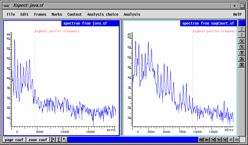
The following image shows two spectra with different upper partial frequencies:
-a attack_smoothing_duration
-r release_smoothing_duration
When a partial starts or disappears in the middle of the sound, its sudden apparition/disparition can be heard as a "clik" or at least as some disturbing sound. To avoid this, its amplitude is smoothed on a a time segment of duration attack_smoothing_duration/release_smoothing_duration given in seconds. Example -a 0.02. Default is 0.05 sec.
-w window type
This option allows selection of the type of analysis window to be used in the fft of the soundfile. "b" specifies blackman, "h" specifies hanning.
-wf0 window type for fundamental
This option allows selection of the type of analysis window to be used in the f0 calculation of the soundfile. "b" specifies blackman, "hn" specifies hanning and "hm" specifies hamming.
-c width_for_seeve_bands
Example -c 0.25. The second step of the complete analysis
(see above) sorts peaks in the neighborhood of harmonic frequencies of
the fundamental frequency f0. This neighborhood is defined by the value
of the width_for_seeve_bands given after the otion -c. More
precisely, let us say that c is the value of width_for_seeve_bands,
then a peak is considered as belonging to the trajectoy of the nth
harmonic partial if it is the peak with maximum amplitude the frequency
fn of which verifies: (n-c).f0 < fn <
(n+c).f0.
NOTE: It seems that at the date 'Wed Apr 5 18:56:44 MET DST 2000',
the formula which is used is instead (n-c*2).f0 < fn <
(n+c*2).f0. If so, it should be corrected! Take care!
Default is 0.5 which means that the band around n.f0 covers half
of the space between (n-1).f0 and (n-1).f0 and half of the space between
n.f0 and (n+1).f0; this means also that all frequencies are covered. A
smaller c constraints harmonic partials to be closer to n.f0. A value
greater than 0.5 is meaningless and should not be used.
-q max_number_of_harmonics
This value indicates the maximum number of harmonic partials written in the parameter file. Default is all the partials. Example -q 20.
-n noise floor for .f0 detection
This value specifies the noise floor to be used when calculating the fundamental frequency for the soundfile. Default value is 40dB.
The following options are executed by the program estimate.-Eb Break_Frequency (default : linear)
In case of spectral envelope estimation, use a logarithmic frequency scale above Break_Frequency Hz for computing the envelope; for frequencies inferior to Break_Frequency, a linear frequency scale is used (default: linear).
-Eo Order
In case of spectral envelope estimation of sinusoidal partials, this option specifies the value of the cepstre Order (default : 50).
-EO Order
In case of spectral envelope estimation of noise, this option specifies the value of the lpc Order (default : 50)
-Er regularization_factor
In case of spectral envelope estimation of sinusoidal partials, this option specifies the value of the regularisation_factor (default:0.00005 ).
-Enum NumEnv
In case of spectral envelope estimation of sinusoidal partials, this option specifies the number of points NumEnv of the estimated envelope (default:128).
-EM Freq
In case of spectral envelope estimation of sinusoidal partials, Freq defines the upper limit of the band [0,Freq] relative to which the cepstral coefficients are calculated. Furthermore, only the partials with frequency lower than Freq are considered in the estimation.
-ENUM NumEnv
In case of spectral envelope estimation of noise, this option specifies the number of points NumEnv of the estimated envelope (default:128).
-EWs WindowSize
In case of spectral envelope estimation of noise, this option specifies the window size for lpc estimation (default :1024 points).