

Next: Further work
Up:
Neural networks for
Previous: Neural models
We have applied our method to various music and speech signals and
present the results for a single saxophone tone, consisting of 16000
samples sampled at 32kHz. For training the signal is normalized
within the range  and the control input t is linear
increasing from
  to
to  . For the following results
  has been used. The time series has been analyzed to estimate the
fractal dimension of the underlying attractors
[Grassberger and Procaccia,
1983]. We obtain a fractal dimension
 , which due to the instationary dynamics has to be
interpreted as an upper limit for the dimension of the generating
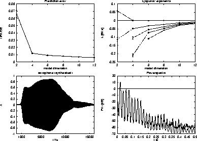
attractors. In fig. 1 we show the relation between input
dimension and prediction error
 of the models.
According to the reconstruction theorem the prediction error nearly
remains constant for
  .
.
Besides the fractal dimension of the attractor its Lyapunov exponents
are important to describe the dynamics. The Lyapunov exponents measure
the sensitivity of the trajectories of the system to small
perturbations. They are mainly used to analyze wether the system
dynamics are chaotic, which is indicated if at least the largest
Lyapunov exponent is positive [Eckmann and Ruelle, 1985]. Similar as in
[Röbel, 1995] we estimate the Lyapunov exponents of the saxophone
models. Due to the instationarity of the models the results estimate
the average Lyapunov exponents for the sequence of attractors. In
fig. 1 we show the largest 5 Lyapunov exponents and realize
that for training on an embedding of the attractors,  , the
largest Lyapunov exponent is zero. Therefore, we conclude that the
dynamics generating the tone at hand are not chaotic.
The most demanding task for the models is the resynthesis of the music
time series. From our systematic investigations we found that for
synthesis purposes the saxophone models need higher input dimension
 . With 200 hidden units these models are capable to
resynthesize the input signal with high quality and, by variation of
the control sequence, does even allow considerable variations of
synthesized sounds. The resynthesized time series and the power
spectra of the original and resynthesized signal are shown in
fig. 1. From the spectrum we see the close resemblance of
the sound. As an example for possible sound control we may invert the
control sequence, such that the sound is synthesized reverse in time,
or fix the control input for some time to generate longer duration of
the tone. At the conference we will give acoustical demonstration of
the synthesized signals.

Figure 1:
Prediction error and the largest 5 Lyapunov exponents of the
saxophone models with varying dimension  . Synthesized saxophone
signal and the powerspectrum estimation for the original
original sound (solid) and the resynthesized sound (dashed).


Next: Further work
Up:
Neural networks for
Previous: Neural models
Axel Roebel
Mon Jul 31 15:37:17 MET DST 1995
 and the control input t is linear
increasing from
  to
to  . For the following results
  has been used. The time series has been analyzed to estimate the
fractal dimension of the underlying attractors
[Grassberger and Procaccia,
1983]. We obtain a fractal dimension
 , which due to the instationary dynamics has to be
interpreted as an upper limit for the dimension of the generating
attractors. In fig. 1 we show the relation between input
dimension and prediction error
 .
.
 , the
largest Lyapunov exponent is zero. Therefore, we conclude that the
dynamics generating the tone at hand are not chaotic.
 . With 200 hidden units these models are capable to
resynthesize the input signal with high quality and, by variation of
the control sequence, does even allow considerable variations of
synthesized sounds. The resynthesized time series and the power
spectra of the original and resynthesized signal are shown in
fig.
 . Synthesized saxophone
signal and the powerspectrum estimation for the original