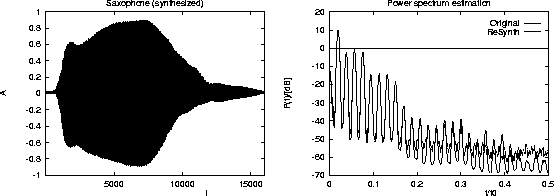
Figure: Synthesized saxophone signal and power spectrum estimation for the original (solid) and synthesized (dashed) signal.
In the following we consider the results for the saxophone model. The
model we present consists of 10 input units, 200 hidden units and 5
output units and was trained with additional Gaussian noise at the
input. The standard deviation of the noise is 0.0005 and the RMS
training error obtained is 0.005. The resulting saxophone model is
able to resynthesize a signal which is nearly indistinguishable from
the original one. The resynthesized time series is shown in
figure
One major demand for the practical application of the proposed musical
instrument models is the possibility to control the synthesized sound.
At the present state there exists only one control input to the model.
Nevertheless, it is interesting to investigate the effect of varying
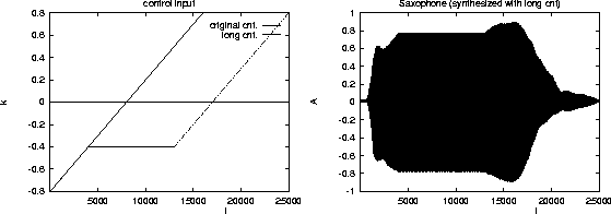
the control input of the model. We tried different control input
sequences to synthesize saxophone tones. It turns out that the model
remains stable such that we are able to control the envelope of the
sound. An example of a tone with increased duration is shown in
figure

Figure:
Synthesized saxophone signal and power spectrum estimation for
the original (solid) and synthesized (dashed) signal.

Figure:
Varying the synthesized tone by varying the control input sequence.