4.4 Discrete Cepstrum Spectral Envelope

Contrary to the previous two methods, LPC, which is computed from the signal, and cepstrum, which is computed from a spectral representation of the signal with points spaced regularly on the frequency axis, the discrete cepstrum spectral envelope is computed from discrete points in the frequency/amplitude plane. These points, which do not have to be regularly spaced in frequency, are the spectral peaks of a sound, which will most often be the sinusoidal partials found by additive analysis (see section 2.2).

As described at the end of sections 3.2 and 3.3, the LPC or cepstrum spectral envelopes will both exhibit the problem to descend down to the level of residual noise between partials which are spaced too far apart, as can be seen in figures 3.3 and 3.6.

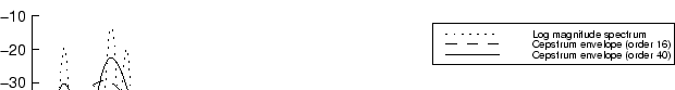
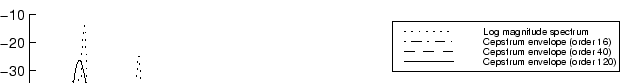
The discrete cepstrum , to the contrary, will not care for anything going on in the signal except the partials. It will generate a smoothly interpolated curve which tries to link the partial peaks, as in figure 3.7.

 

tex2html_comment_mark>

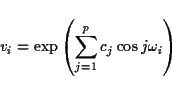
The following method to estimate the discrete cepstrum was developed by Thierry Galas and Xavier Rodet in [GR90,GR91a,GR91b]. A given set of spectral peaks (partials) with amplitudes x_i at frequencies $\omega_i, i = 1..n$, defines a magnitude spectrum X as

$$X = \sum_{i=1}^n {x_i\delta(\omega_i)}$$

We consider X to be the result of a convolution

$$X = S \* P$$

where S is the source spectrum with amplitudes s_i at the same frequencies $\omega_i$ as for X

$$S = \sum_{i=1}^n {s_i\delta(\omega_i)}$$

and P is a filter transfer function of a filter modeled by

$$P (\omega) = \prod_{i=0}^p {e^{c_i \cos \omega i}}$$

Assuming a flat source spectrum $S(\omega) = 1$ for all $\omega$, all we need to do is find the filter parameters c_i which minimize the quadratic error E between the log spectra. This error criterion is developed from the idea of a spectral distance.

   $$E = \sum_{i=1}^n {\left( \log s_i P(\omega_i) - \log x_i \right)^2}$$

To achieve this, one has to simply solve the matrix equation

  A c = b

where A is a matrix of order p+1, where p is called the order  of the discrete cepstrum, given by

   $$a_{ij} = \sum_{k=1}^n {\cos \omega_k i \ \cos \omega_k j}$$

c is the vector of filter parameters we're looking for

$$c = \left( \begin{array}{c} c_1 \\ \vdots \\ c_p \end{array} \right)$$

and b ist the column vector given by

   $$b_i = \sum_{k=1}^n {\log \frac{x_k}{s_k} \cos \omega_k i}$$

The matrix A can be computed very efficiently by using an intermediate vector R given by

$$r_i = \frac{1}{2} \sum_{k=1}^n {\cos \omega_k i}$$

so that a_ij = r_i+j - r_i-j.

The matrix equation (3.18) can be efficiently solved applying the Cholesky algorithm , which factorises A such that

$$A = U D \,\, U'$$

where U is an inferior triangular matrix  whose diagonal elements are 1, U' is the transposed matrix (i.e. it is a superior triangular matrix , and D is a diagonal matrix. Now the matrix equation can be solved by simple substitution and division.

The asymptotic complexity of the discrete cepstrum method described above is O(np + p³), which means that the number of partials n is not of a big concern, since the order is linear in n, but that the order p has to be kept as small as possible, because of its cubic influence.