The issue of time deformation can be seen more generally in the light of the representation of continuous time. Of course, no such thing as continuous time exists in digital systems. However, we have defined our control functions such that their value can be requested at any time value (section 5.3). It is in this fashion that we interpret the notion of ``continuous'' time functions in this text. Our proposition for the manipulation and integration of continuous time is a combination of Honing & Desain's generalized time functions [Hon93] and time warping, in particular Dannenberg's work [Dan97]. Other works relevant to this discussion are those by Rodet & Cointe [RC84], and Anderson & Kuivila [AK89].

The layered time models coincides with the structural hierarchy described by patterns and motifs. This rich time representation is used to transform the start times and durations of activities and to describe non-linear dependencies of control functions on absolute time.

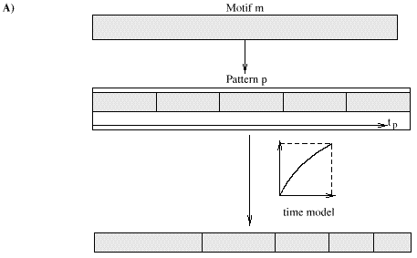
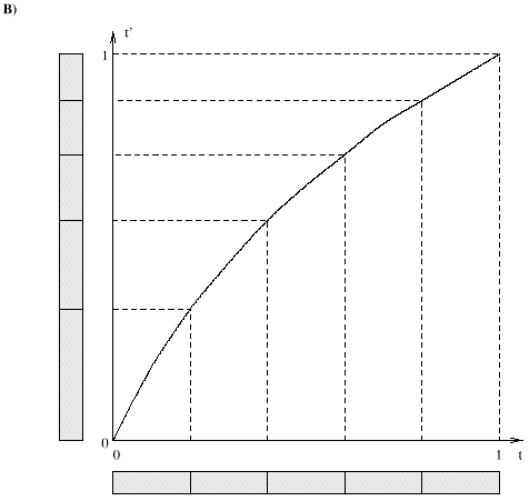
Figure 6.7: The figure shows an example of a time model. A) Above is depicted the original pattern and motif as it is used in the composition. Below are shown the activities with their final durations after scheduling. B) The start times and the durations of the activities are mapped using the time model.

To the hierarchy of motifs and patterns will we attach a hierarchy of time models. Consider figure 6.7. Motif msubscribes to pattern p. When motif m requests its contents, pclones its contained activities and organizes them according to m's duration. We will introduce a virtual time axis t_p for pattern p. In reality p has no such time axis. This axis only exists when p organizes the activities for a particular motif. In that case the length of the time axis is the duration of the motif. Once the activities are organized, their start times and the durations are mapped from p's virtual time axis onto m's time axis. For this mapping pattern p uses a time model. The example in figure 6.7 depicts a logarithmic time model. This time model provokes an accelerando. Time models are defined as follows:

Definition 2 (Time model) A time model tm is a bijection that maps a value t onto a value t': tm: [0,1]->[0,1], t'=tm(t). TM denotes the set of time models. A special time model is the linear model, tm_linear: t' = t.

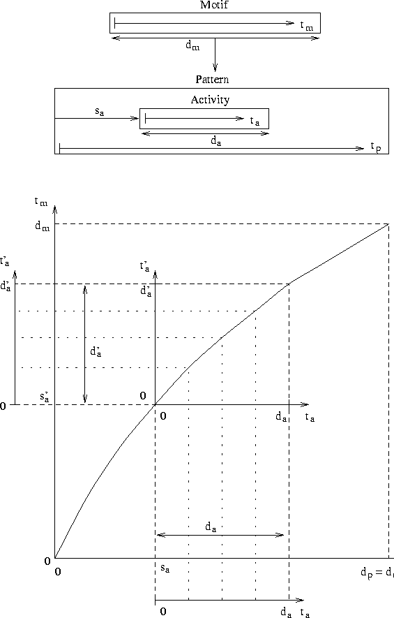
Figure 6.8: Figure a) shows a simple organization. Motif m and activity a have a local time axis. Both axes stand in some relationship to each other. This relationship is described by the time model of pattern p. B) Time models describe the mapping of the time axis of an activity onto the time axis of a motif.

Time models are not only used to adjust the start position and durations of the activities. With every activity we associate a local time axis (see figure 6.8). Motif m has a local time axis t_m, and activity a has a local time axis t_a. These two axes stand in some relationship to each other. This relationship is described by the time model of the pattern p that contains a. How this relationship is articulated is shown in the figure. For the construction of this relationship we will rely on p's virtual time axis t_p. The mapping of the time axis of activity a onto the time axis of motif m requires the time model of the pattern p and the offset and duration of a. When we let the time grow linearly on the time axis of a, it will grow logarithmically on m's time axis. Vice versa, when the time advances linearly on axis t_m, t_a grows exponentially.

Figure 6.9: Any synthesis process created by an activity is embedded in a time context. This time context describes the time dependencies, as defined in the composition, between the local time axis and the real time.

When the activities are scheduled, they will provoke the creation of new synthesis processes (see also figure 6.6). These synthesis processes and the control functions that steer them must experience the same time dependencies as the activities in the composition. We must therefore pass all the time information and the context in which the activity finds itself in the composition to the synthesis processes and their control functions. We will group this information in a structure called time context (Fig. 6.9). This time context ensures the correct conversion from the real time to the local time of the synthesis process.

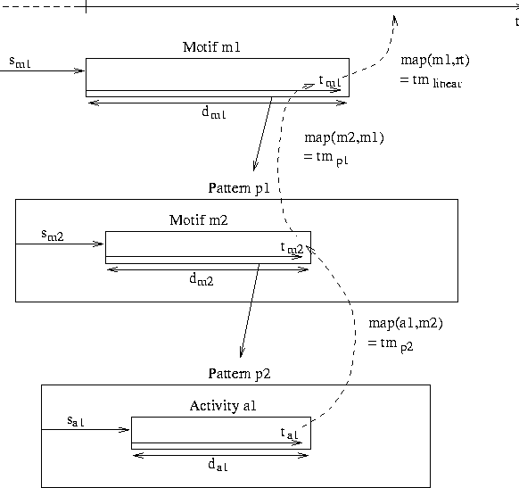
Consider figure 6.10. An activity a1 starts at a time s_a1 and has a duration d_a1. Both s_a1 and d_a1 are measured on the time axis of a₁'s pattern p2. When a₁ is performed, it experiences a time t_a1. Motif m₂subscribes to the organization of pattern p₂ and is included into the pattern p₁. It has a start time s_m2 and duration d_m2measured on the time axis of p₁. When motif m₂ is performed, it experiences a time t_m2. Motif m₁ subscribes to the organization of pattern p₁ and has a duration d_m1. When the user request the performance of motif m₁ at some time s_m1, activity a₁ will be scheduled at its appropriate time. The mapping of the time experienced by the activity a₁ onto the real time dictated by the system depends on the start times of a₁, m₂, and m₁, and the time models of p₂ and p₁. The mapping of t_a1 onto t_m2 is described by the time model of p2. The mapping of t_m2 onto t_m1 is described by the time model of p1. A synthesis process created by the activity a₁ must be able to reconstruct this hierarchy of time dependencies during the performance. For this purpose, we chain the necessary data into a series of time contexts.

Definition 3 (Time context) A time context c is a quadruple <s,d,tm,c'>. s in R₊ indicates an offset time, d in R₊ a duration, tm in TM a time model. c' is the parent time context of c.

In the case of activity a₁ in figure 1.9 the context c is equal to <s_a1,d_a1,tm_p2,c'>. c' is the parent time context of a₁, i.e. the time context of motif m₂.

Figure 6.11: Any synthesis process created by an activity refers to a linked list of time contexts. The synthesizer passes the synthesis process the real clock time. Using this time and the contexts, the process can calculate the time on any level of its parent's contexts.

We can now fully specify the interfaces of the synthesizer object and of the activities. The add method of the synthesizer expects three arguments:

When activity a₁ is scheduled, its start program p_s is invoked. The first arguments passed to p_s is the time context c of a. c holds a reference to its parent time context, and so forth. The argument passed to p_s is thus a chained list of time contexts (Fig. 6.11). p_s creates a new synthesis process sp and adds it to the synthesizer passing along the time context. When the synthesizer calls the synthesis process sp it converts the absolute time indicated by the system to the local time of the synthesis process using sp's time context. When the synthesizer calls the synthesis process to produce the sound, it gives as parameters the synthesis buffer, the local time, and the time context. sp calls upon any control function with its local time and, again, the time context. Using this local time and time context, the control functions can calculate the time on any superior time level of the composition. This possibility will be used in the example of amplitude curves, portamento, and vibrato discussed in section 6.7. First, we take a closer look at activities used for sound production.